Sentiment Analysis using R – Lego Batman Movie
The Lego Batman Movie is a 3D computer-animated superhero comedy film released in 2017. The movie had 430,000+ followers on Facebook (as on Apr 2017). The movie was released on 17 Feb 2017 so we would like to analyse the sentiment of this movie post release.
I will be using two kind of approaches for text-mining tweets
- Approach 1: Using ‘tm’ package – this is a basic text -mining framework package available in R
- Approach 2: Using ‘syuzhet‘ package – this package is built on top of core NLP package that comes with advanced sentiment extraction tools
Tweet Extraction
The tweets were read through Twitter API directly in R. You can refer to great tutorial by 'Credera: Twitter Analytics Using R Part 1: Extract Tweets' for extracting tweets.
Tweet Pre-processing
Loading Libraries
You'll need the following libraries to pre process the tweets.
- stringr - gives access to chararcter manipulation, whitespace tools, pattern matching and case transformation functions
- readr - for reading rectangular datasets
- wordcloud - to generate a beautiful wordcloud.
- tm - the weighlifting text mining package
- SnowballC - to implement Porter’s word stemming. Stemming refers to find a common root the words like, running, run are have run as their root
- RSentiment - reads sentence sentiments in English in five categories namely Positive, Negative, very Positive, very negative, Neutral
library('stringr')
library('readr')
library('wordcloud')
library('tm')
library('SnowballC')
library('RWeka')
library('RSentiment')
library(DT)
library(ggplot2)
Loading Dataset
The scraped tweets were saved as .csv file. Each tweet items has features like name, retweet, tweet text, URL etc. For the purpose of sentiment analysis, we will use tweet text only.
tweets = read_csv("tweets.csv")
tweets_text = as.character(tweets$text)
Pre-Processing
The tweet text contains links, numbers, punctuation, emojis, white space, and related words that can be stemmed. The operations are done in the following code.
sample = sample(tweets_text, (length(tweets_text)))
corpus = Corpus(VectorSource(list(sample)))
corpus = tm_map(corpus, removePunctuation)
corpus = tm_map(corpus, content_transformer(tolower))
corpus = tm_map(corpus, removeNumbers)
corpus = tm_map(corpus, stripWhitespace)
corpus = tm_map(corpus, removeWords, stopwords('english'))
corpus = tm_map(corpus, stemDocument)
dtm_up = DocumentTermMatrix(VCorpus(VectorSource(corpus[[1]]$content)))
freq_up =
Computing Sentiments
sentiments_up = calculate_sentiment(names(freq_up))
sentiments_up = cbind(sentiments_up, as.data.frame(freq_up))
sent_pos_up = sentiments_up[sentiments_up$sentiment == 'Positive',]
sent_neg_up = sentiments_up[sentiments_up$sentiment == 'Negative',]
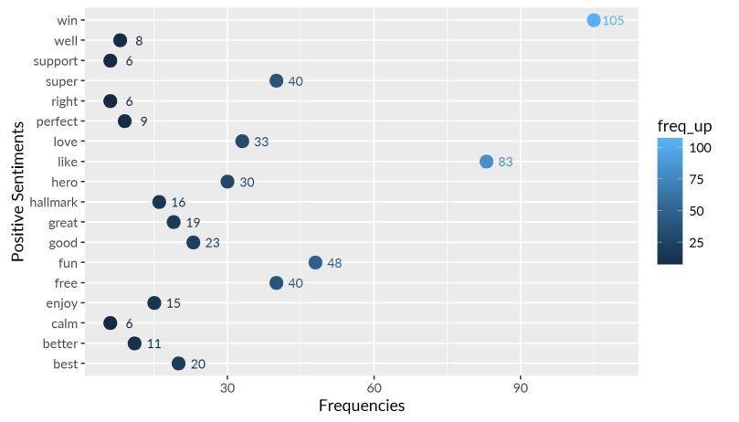
Plotting Positive Sentiments
For aesthetics I used a Windows font
windowsFonts(Lato.Regular = windowsFont('Lato Regular'))

 # PLotting the positive sentiments
 ggplot(aes(x = freq_up, y = text, label = freq_up, color=freq_up),
 data = sent_pos_up[sent_pos_up$freq_up>5,]) +
 geom_point(size=4) +
 geom_text(size=3,
           position = position_nudge(x = 4),
           family = "Lato.Regular") +
 theme_gray(base_family = "Lato.Regular") +
 ylab("Positive Sentiments") +
 xlab("Frequencies")
The output shows that win is the most frequent word. The words in the graph below are limited by their frequencies. Words that appear more than 5 times in the term-document matrix are plotted here.
Word Cloud
## Wordcloud positive sentiments
layout(matrix(c(1, 2), nrow=2), heights=c(1, 4))
par(mar=rep(0, 4))
plot.new()
wordcloud(sent_pos_up$text,sent_pos_up$freq,min.freq=5,colors=brewer.pal(6,"Dark2"))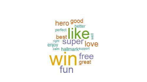
Plotting Negative Sentiments
ggplot(aes(x = freq_up, y = text, label = freq_up, color=freq_up),
       data = sent_neg_up[sent_neg_up$freq_up>5,]) +
  geom_point(size=4) +
  geom_text(size=3, position = position_nudge(x = 4), family = "Lato.Regular") +
  theme_gray(base_family = "Lato.Regular") +
  ylab("Negative Sentiments") +
  xlab("Frequencies")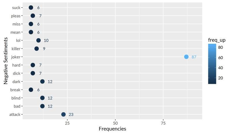
Wordcloud of Negative Sentiments
layout(matrix(c(1, 2), nrow=2), heights=c(1, 4))
par(mar=rep(0, 4))
plot.new()
set.seed(100)
wordcloud(sent_neg_up$text,sent_neg_up$freq, min.freq=5,colors=brewer.pal(6 ,"Dark2"))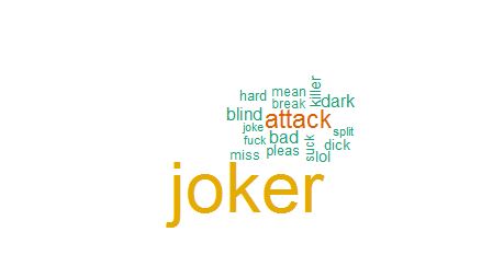
Approach 2: Using 'syuzhet' package
‘Syuzhet’ essentially means the manner in which the elements of the story are organised. The package in R does so by revealing the latent structure using sentiment analysis. It considers 9 emotional expressions excluding positive and negative sentiments.
So start we need to first load the .csv file and extract the text only.
text = as.character(tweets$text)Data Pre-processing
Now the data is loaded we need to take care of HTML tags, punctuations, username, retweets and numbers. Let’s remove them one by one.
##removing Retweets
some_txt = gsub("(RT|via)((?:\\b\\w*@\\w+)+)","",text)
##let's clean html links
some_txt = gsub("http[^[:blank:]]+","",some_txt)
##let's remove people names
some_txt = gsub("@\\w+","",some_txt)
##let's remove punctuations
some_txt = gsub("[[:punct:]]"," ",some_txt)
##let's remove number (alphanumeric)
some_txt = gsub("[^[:alnum:]]"," ",some_txt)
Calculating Sentiment score
Once the data is cleaned, we are ready to calculate sentiment score for each emotion
library(syuzhet)
mysentiment = get_nrc_sentiment((some_txt))
mysentiment.positive =sum(mysentiment$positive)
mysentiment.anger =sum(mysentiment$anger)
mysentiment.anticipation =sum(mysentiment$anticipation)
mysentiment.disgust =sum(mysentiment$disgust)
mysentiment.fear =sum(mysentiment$fear)
mysentiment.joy =sum(mysentiment$joy)
mysentiment.sadness =sum(mysentiment$sadness)
mysentiment.surprise =sum(mysentiment$surprise)
mysentiment.trust =sum(mysentiment$trust)
mysentiment.negative =sum(mysentiment$negative)
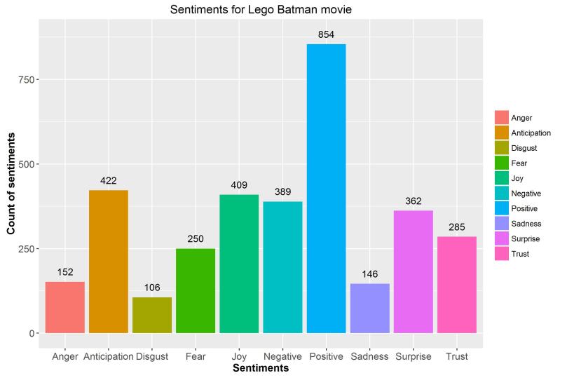
Sentiment Plot
In the plot, there are a higher number of positive sentiments forllowed by anticipation, owing the the fact that the tweets were taken just a few days after the movie was released and hence people were anticipating the movie would be good. The movie was intented to be funny, which is reflected in the chart as 'Joy' being the third leading sentiment.
Conclusion
Using both ‘tm’ and ‘syuzhet’ package it turns out that lego batman movie had a higher number of positive sentiments than the negative ones. This means that movie was well received by the audience. Also one could also notice that most negative sentiments were also related to the joker
As it turns out that movie is not looking for positive sentiments only, one can define the success of the movie by scoring the negative sentiments too. Because in the end, that is what lego batman movie wanted to achieve. The higher number of negative sentiments on joker is a true indicator of the success of the movie.