The TorchVision Playground

Think about how a photo gets ready before it's printed or posted online:

• It gets cropped to fit the frame.
• It's resized to the right dimensions.
• Maybe it's brightened up a little.

Before an AI model can look at a photo and say "that's a flower," it goes through a similar prep process. The photo gets:

• Resized.
• Cropped.
• Turned into a grid of numbers the model can actually read.
• Rescaled, so those numbers fall in a consistent range.

To teach a model to learn to see flowers, showing the same flowers can lead to:

• Memorizing those specific photos instead of learning features
• Difficulty in identifying new photos even if the angle / bridghtness is changed slightly

So to make the model learn to see flowers, each photo also gets randomly flipped, rotated, or recolored a little differently every time it's shown. This trick is called augmentation. It forces the model to learn the idea of "flower", and focus on the underlying features that make up a flower

This whole sequence of steps is an image processing pipeline. Nearly every large image AI you've used like ChatGPT, Nano Banana, Midjourney is built on a pipeline just like this one. This is made possible by one very cool library called TorchVision.

What You Will Learn

In this article, you will learn about the TorchVision library and the set of tools that it offers that make up the image processing pipeline. It offers:

• Transforms: to prepare and randomize your images
• Datasets: to load and test with image data
• Models: pretrained networks for classification, detection, and segmentation
• Utils: utilities to visualize the results

Let's get to it!

Deep learning for computer vision comes with a lot of hidden work — loading images, augmenting them, normalizing them, batching them, defining models, and visually debugging all of it. Writing that from scratch is slow, error-prone, and a pain to maintain.

TorchVision packages all of it into one library instead. Using it gives you:

• Consistency — it plugs straight into PyTorch's components like Dataset and DataLoader.
• Efficiency — many transforms are optimized in C or TorchScript, not plain Python.
• Reliability — standardized code means fewer bugs and results you can reproduce.

That lets you spend your time on your own computer vision problem, instead of reinventing tools that already exist. TorchVision provides those tools in four key areas:

The sections below work through the transforms, the utilities, and the datasets:

Setting up the Environment

from PIL import Image  # For Image I/O
import torch
from torchvision import transforms

torch.manual_seed(42)                   # Helps with reproducibility
img = Image.open("flower-1.jpg")        # PIL image · H × W × C
H, W = img.height, img.width            # PIL gives channels-last size
C = len(img.getbands())                 # e.g. 3 for RGB
print(f"Image Size: {H} x {W} x {C}")

TorchVision's transforms module is built around five core functions — ToTensor(), ToPILImage(), Resize(), CenterCrop(), and Normalize(). The first two helps you convert an image to a tensor and back

• ToTensor() — converts an image from PIL (Pillow) format into a PyTorch tensor, scaling pixel values from the 0–255 range down to 0–1 — which helps stabilize training by keeping inputs consistent. The resulting tensor is in CHW format (channels, height, width), unlike NumPy and PIL, which use HWC format (Height, Width, Channels)
• ToPILImage() — converts a tensor back into a PIL image. The image comes back unchanged, with no deterioration — a 2048×2048 image stays 2048×2048.

Hover the image below to see a pixel's raw values before and after that conversion.

# ToTensor(): PIL → tensor · uint8 [0,255] HWC → float32 [0,1] CHW
tensor = transforms.ToTensor()(out)

# ToPILImage(): the exact inverse — tensor → PIL, back to the original image
back = transforms.ToPILImage()(tensor)

Preprocessing involes resizing, cropping and normalizing images before they are fed into a model. TorchVision provides three core transforms for this purpose:

• Resize() — adjusts the input image to a specific size, ensuring consistent input dimensions. If the image isn't square, the smaller edge is resized first and the other edge is proportionally resized. Reducing resolution (e.g., to 50×50) makes the image look pixelated.
• CenterCrop() — captures the image's central portion after resizing and removes irrelevant edges. Both Resize() and CenterCrop() take the desired output size as an argument.
• Normalize() — after pixel values are in the 0–1 range, channels are normalized to have a mean of 0 and a standard deviation of 1, by subtracting the mean and dividing by the standard deviation for each channel — essentially computing the z-score.

transform = transforms.Resize(224)

transform = transforms.Compose([
    transforms.Resize(256),
    transforms.CenterCrop(224),
])

transform = transforms.Compose([
    transforms.ToTensor(),                 # Normalize needs a tensor first
    transforms.Normalize(mean=[0.485, 0.456, 0.406],
                         std=[0.229, 0.224, 0.225]),
])

A small dataset is the usual reason to augment: each random variation is effectively a new training sample, teaching the model that the label survives the change. The Random* transforms roll fresh dice on every call — here the dice are a seed you control, the same trick as torch.manual_seed(). Same seed, same "random" result.

torch.manual_seed(7)
transform = transforms.ColorJitter(brightness=0.4, contrast=0.4, saturation=0.4)

torch.manual_seed(7)
transform = transforms.RandomHorizontalFlip(p=0.5)

torch.manual_seed(7)
transform = transforms.RandomResizedCrop(224, scale=(0.30, 1.0))

If you want to implement your custom tranforms, TorchVision allows it. It only requires the function you write is callable. The classic example: salt-and-pepper noise, random white and black pixels simulating a grainy sensor.

class SaltAndPepperNoise:
    def __init__(self, ratio=0.5, amount=0.05):   # parameters live here
        self.ratio, self.amount = ratio, amount
    def __call__(self, img):                      # the operation lives here
        arr = np.array(img)
        n = int(arr.shape[0] * arr.shape[1] * self.amount)
        ys, xs = np.random.randint(0, arr.shape[0], n), np.random.randint(0, arr.shape[1], n)
        arr[ys, xs] = np.where(np.random.rand(n, 1) < self.ratio, 255, 0)
        return Image.fromarray(arr)

transform = SaltAndPepperNoise(ratio=0.5, amount=0.050)

Compose() combines multiple transforms into a single preprocessing pipeline defined as a list of operations applied in sequence. Any image passed through will come out the correct size, format, and scale. Because everything is defined in one place, it's easy to reuse and maintain consistency across datasets.

When you pass a pipeline to a TorchVision dataset, the transformation is automatically applied to every image entering a batch.

Process — a typical preprocessing pipeline:

1. Resize() the image.
2. CenterCrop().
3. ToTensor().
4. Normalize() using the ImageNet mean and standard deviations.

Pipelines built with Compose() help solve a common challenge: a small dataset. Even with a good architecture, limited data may be too little to train effectively. One solution is to create variations of each image — color jitter, rotation, noise, random crops, random resizing. This is image augmentation: each new version effectively becomes a new sample, increasing data size and variety without collecting new data.

Common random transformations include:

• RandomResizedCrop() — randomly crops and resizes different parts of the image (e.g., to 224×224), encouraging the model to focus on all object areas, not just the center.
• RandomHorizontalFlip() — randomly flips images horizontally (default probability 0.5), helping the model learn that objects can appear in either direction.
• ColorJitter() — randomly adjusts brightness, contrast, and saturation (e.g., by a factor randomly selected between 0 and 0.5) to make the model more resilient to lighting variations.

After applying random transforms, convert images to tensors and then normalize.

The cards below are those stages in order — follow the arrows. Drag a card to reorder it, press × to remove it, and add more from the tray. If you put, Normalize() before ToTensor() and you would get an error.

Using make_grid to Visualize multiple transformations at once and save_image() exports tensors back into image file formats like JPEG or PNG.

from torchvision.utils import make_grid, save_image

batch = torch.stack([transform(img) for _ in range(6)])
grid  = make_grid(batch, nrow=3, padding=4, normalize=True)
save_image(grid, "contact_sheet.png")

Bounding boxes are a key output of object detection models, indicating the locations and categories of objects. Visualizing them helps you understand and validate predictions

Process — drawing boxes manually:

1. Import the utilities module (contains draw_bounding_boxes).
2. Create bounding boxes with coordinates x1, y1, x2, y2, defined as a tensor (hard-coded here).
3. Define corresponding labels.
4. Call draw_bounding_boxes with the image tensor, box coordinates, and labels → a new tensor containing the annotated image.

The boxes in the previous station were hand-placed. In practice the coordinates come from a detection model, and draw_bounding_boxes paints them exactly the same way.

Process — drawing boxes from a pretrained model:

1. Use Faster R-CNN with a ResNet50-FPN backbone — Faster R-CNN for region proposal and classification, ResNet50 for feature extraction, and a feature pyramid network to detect objects at multiple scales. It's pre-trained on COCO (detects a wide range of common objects).
2. Load the model and set it to evaluation mode.
3. Check which classes it can detect — per the documentation, 90 object categories plus a background class (10 are labeled NA); "car" and "traffic light" are included. A helper function reads the metadata to retrieve categories.
4. Load the image; specify target classes (e.g., "car", "traffic light") and box colors (red for cars, blue for traffic lights).
5. Define detect_and_draw_bboxes(), which converts the image to a tensor, runs it through the model, and retrieves predictions with box coordinates, class labels, and confidence scores.
6. Filter predictions to those matching the target classes above a confidence threshold; overlay the filtered boxes with draw_bounding_boxes, customizing line color and thickness. Return the annotated tensor (or the original image if nothing was detected above threshold).
7. Call detect_and_draw_bboxes() with the model, image path, target category indices, box colors, and a confidence threshold of 0.7.

load_the_detector.py

# Load a pre-trained object detection model and set to evaluation mode
bb_model_weights = tv_models.detection.FasterRCNN_ResNet50_FPN_Weights.DEFAULT
bb_model = tv_models.detection.fasterrcnn_resnet50_fpn(weights=bb_model_weights).eval()

# Use the helper function to inspect the weights object of the object detection model.
num_classes, classes = get_model_classes_from_weights_meta(
    model=bb_model,
    weights_obj=bb_model_weights
)

target_classes.py

# Define a list of target classes to detect
target_class_names = ['car', 'traffic light']

# Define a corresponding list of colors for each class's bounding box
bbox_colors = ['red', 'blue']

# Use a list comprehension to get a list of all target indices
object_indices = [classes.index(name) for name in target_class_names]

detect_and_draw_bboxes.py

def detect_and_draw_bboxes(model, image_path, object_indices, labels, bbox_colors,
                           threshold, bbox_width=3):

    # Open and transform the image, and prepare the result tensor
    pil_image = Image.open(image_path).convert("RGB")
    transform_to_tensor = transforms.Compose([transforms.ToTensor()])
    tensor_image_batch = transform_to_tensor(pil_image).unsqueeze(0)
    result_image_tensor = (tensor_image_batch.squeeze(0) * 255).byte()

    # Perform inference to get predictions for all possible objects
    with torch.no_grad():
        prediction = model(tensor_image_batch)[0]

    # Initialize lists to collect all boxes, labels, and colors that meet the criteria
    all_boxes_to_draw = []
    all_labels_to_draw = []
    all_colors_to_draw = []

    # Loop through each target class to find its boxes
    for index, label, color in zip(object_indices, labels, bbox_colors):
        # Filter predictions for the current class index and confidence threshold
        class_mask = (prediction['labels'] == index) & (prediction['scores'] > threshold)

        # Get the boxes for the current class
        boxes_for_this_class = prediction['boxes'][class_mask]

        if boxes_for_this_class.nelement() > 0:
            # Add the found boxes to our master list
            all_boxes_to_draw.extend(boxes_for_this_class.tolist())
            # Create and add corresponding labels and colors
            all_labels_to_draw.extend([label] * len(boxes_for_this_class))
            all_colors_to_draw.extend([color] * len(boxes_for_this_class))

    # After checking all classes, draw all collected boxes at once if any were found
    if all_boxes_to_draw:
        result_image_tensor = vutils.draw_bounding_boxes(
            result_image_tensor,
            torch.tensor(all_boxes_to_draw),
            labels=all_labels_to_draw,
            colors=all_colors_to_draw,
            width=bbox_width
        )
    else:
        # If the list of boxes to draw is empty, print this information.
        print(f"No objects from the list {labels} were found with a confidence score above {threshold}.\n")

    return result_image_tensor

run_detection.py

confidence_threshold = 0.7

# Execute the main detection function
result_image_tensor = detect_and_draw_bboxes(
    model=bb_model,                    # The pre-trained object detection model.
    image_path=image_path,             # The path to the input image.
    object_indices=object_indices,     # The list of integer indices for the target classes.
    labels=target_class_names,         # The list of string names for the box labels.
    bbox_colors=bbox_colors,           # The list of colors for the bounding boxes.
    threshold=confidence_threshold,    # The minimum confidence score for a detection.
)

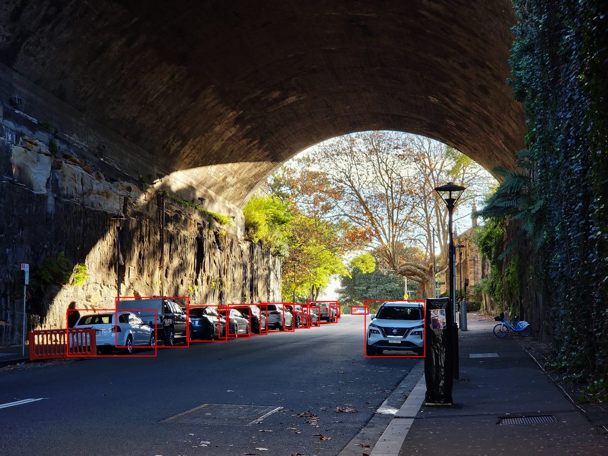
output of detect_and_draw_bboxes() — Faster R-CNN R50-FPN, COCO weights, threshold 0.70: 12 boxes for car, none for traffic light (there are none in frame)

• Three ways TorchVision helps with data:
  • Pre-built datasets — come with labels, formatted to integrate into PyTorch's training pipeline directly. Enable training and comparison against established benchmarks (MNIST, ImageNet), faster deployment, and testing/debugging of models and pipelines.
  • Custom datasets — the most common application; TorchVision offers strong support for loading, pre-processing, and augmenting your own data.
  • Fake (synthetic) datasets — quickly generated to debug pipelines and ensure the data shape stays consistent for your architecture.

• FakeData — generates random images and labels mimicking a real dataset's shape and size. Ideal for testing without worrying about data availability — e.g., confirming your images are the right size for your model.

from torchvision.datasets import FakeData
ds = FakeData(size=8, image_size=(3, 32, 32), transform=transforms.ToTensor())

• Overview of TorchVision tools — datasets, model architectures, transforms, and visualization tools.
• Preprocessing pipelines, including data augmentation — normalizing images, applying augmentations, and implementing custom transforms integrated directly into the training loop.
• Working with built-in and custom datasets — structuring data for seamless integration with PyTorch's DataLoader.
• Pretrained models: inference and transfer learning — loading models, performing inference, and adapting them to new tasks (examples from ResNet and MobileNet).
• Visualization utilities: bounding boxes and segmentation — overlaying boxes or masks to interpret and debug model behavior.
• Together, these tools let you build, train, evaluate, and inspect computer vision models with enhanced clarity and efficiency